Lab Session 2 - Supervised Learning⚓
Objectives of the lab⚓
At the end of this session, you will be able to :
- Perform basic supervised learning tasks using sklearn.
- Apply supervised learning on your chosen application
Note
Whenever possible, we have included links to the official documenation of the functions you need to use. Check them out, you'll save a lot of time !
Prerequisites⚓
You have to do lab 1 before. This includes :
- Knowing how to manipulate numpy arrays, in particular indexing an array using another array
- Knowing how to basic plotting of vectors using
matplotlib.pyplot(1D plots, scatter plots, ...) - Knowing how to load / save numpy arrays
Intro to sklearn⚓
Install scikit-learn using pip. If you need details, see here, but a simple pip install scikit-learn should work.
Note
The package is imported using import sklearn but the actual package name for installation is scikit-learn
Basics of machine learning using sklearn⚓
sklearn is a very powerful package that implements most machine learning methods. sklearn also includes cross-validation procedures in order to prevent overfitting, many useful metrics and data manipulation techniques that enables very careful experimentations with machine learning. It is also very straightforward to use. We will introduce a few basic concepts of sklearn.
First, it is very easy to simulate data with sklearn. In lab 1, we made you code the generation of two point clouds using numpy functions. The make_blobs function does it, with many added options.
1 | |
Use the function make_blobs to generate clouds of points with \(d=2\), and visualize them using the function scatter from matplotlib.pyplot. You can generate as many samples as you want. You can generate several clouds of points using the argument centers. We recommend using random_state=0 so that your results are from the same distribution as our tests.
Vocabulary : n_samples is the number of generated samples, n_features is \(d\) (number of dimensions), centers is the number of classes.
Hint : you can use the output "y" as an argument for the color argument ("c") of the scatter function.
1 | |
You can use other arguments from make_blobs in order to change the variance of the blobs, or the coordinates of their center. You can also experiment on higher dimension, although it becomes difficult to visualize.
sklearn has many other data generators, as well as ways to load standard datasets of various sizes.
Train test Split⚓
Now that we have generated a simple dataset, let's try to do a basic supervised learning approach.
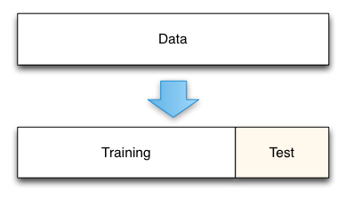
First, in order to mesure the ability of the model to generalize, we have to split the dataset into a training set and a test set. The test set is the part of the dataset that the model will not see during the training and will be used as a proxy for your "real world" examples.
In sklearn, you can use the train_test_split function to split datasets.
Try to split the dataset you previously generated (the blobs) into x_train, x_test, y_train, y_test, with 80% in x_train and 20% in x_test. Set random_state = 0 so that the function always returns the same split.
Check the shapes of the generated vectors.
1 | |
K-Nearest Neighbor⚓
Let's use a K-Nearest Neighbor classifier to test whether we can classify this dataset. Create a classifier, train it using your training set and evaluate it by its accuracy on both the train and test sets.
In K-Nearest Neighbor classification (also known as KNN), when you want to predict the class of an object, you look at the K (an hyperparameter) nearest examples from the training (using a distance metric, in our case the euclidean distance). This object is then classified by a majority vote among its neighbors. In other words, the class of the object is the most common class among its neighbours.
To use a Nearest Neighbor with sklearn, you have to use the class KNeighborsClassifier.
The sklearn API is consistent. This means that for almost every method they propose you can train it using object.fit, you can use it to make prediction with object.predict and finally verify the accuracy of the method using object.score.
1 2 3 4 | |
Your classifier should have a train accuracy of 1, while the test accuracy should be high but not perfect.
This is caused by the bias-variance trade-off. The 1-NN classifier always has a bias of 0 (it perfectly classifies the training set) but it has a high variance given that having one more example in the training set can completely change a decision.
Try to avoid having such a high variance, test different values of k and plot the accuracies given the different values of the hyperparameter k.
If you have time, we advise you to do the same analysis but varying the train/test split size.
1 2 3 4 | |
Precision, Recall and F1-score⚓
Once your classifier is trained, and bias-variance analysed, it is time to look at other metrics based on your results. It is important to remember that accuracy is a key metric, but it is not the only metric you should be focusing on.
Print a classification report and a confusion matrix for both training and test sets.
In the classification report, you are going to see 3 new metrics. They are really important because the accuracy does not show a complete portrait of your results.
- Precision: Percentage of correctly classified examples with respect to all retrieved examples
- Recall: Percentage of correctly classified examples with respect to all examples belonging to a given class
- F1 Score: Harmonic mean from precision and recall.
1 2 | |
Decision Boundaries⚓
Finally, you are going to plot the decision boundaries of our model. Use the function plot_boundaries given below. You can only do this if the tensor representing your data is two dimensional.
This function will test our model with values ranging from the smallest x to the highest x and from the lowest y to the highest y, each varying by \(h\) and plot it nicely. Link to the original implementation.
1 2 3 4 5 6 7 8 9 10 11 12 13 14 15 16 17 18 19 20 21 22 | |
Application⚓
There are three things to do :
- Choose a supervised learning algorithm from the following list :
- Decision Trees -
sklearn.tree.DecisionTreeClassifier - Support Vector Machines -
sklearn.svm.SVC - Logistic Regression -
sklearn.linear_model.LogisticRegression - Adaboost -
sklearn.ensemble.AdaBoostClassifier - Multilayer Perceptron (MLP) -
sklearn.neural_network.MLPClassifier - Random Forest -
sklearn.ensemble.RandomForestClassifier
- Decision Trees -
- Use synthetic data generation, or a simple "toy" dataset, to explain how the algorithm works, and the influence of its hyperparameters.
- Apply this algorithm to your chosen application, by referring to the application pages (section "Ressources for Session 2")
In Session 3, you will have to present these three things in a 7 minute presentation.